
Descriptive Statistics: The Foundation of Forensic Data Analysis
Descriptive Statistics for Digital & Multimedia Forensic Sciences
Let me offer you a new perspective on an old definition: Multimedia forensics is collecting, analyzing, and preserving digital images, videos, audio, and related metadata for legal investigations. It relies on robust statistical foundations to interpret and present evidence accurately and reliably.
Descriptive statistics provide the essential tools to summarize and understand multimedia evidence, as emphasized by Lucy in his comprehensive guide to statistical methods in forensic science [1]. They also support forensic experts in identifying patterns, detecting anomalies, and presenting findings clearly to investigators or in court. By applying these statistical techniques to multimedia data, we ensure our conclusions about audio, image, or video authenticity, tampering, or compression effects are objective, defensible, and well-supported by the evidence.
I wanted to begin a series of blog posts on statistics for digital and multimedia forensics. While the underlying statistical methods we will discuss are not unique to our field, I aim to emphasize how these standard statistical tools are vital for digital and multimedia forensic sciences while helping experts make sense of complex evidence and communicate their findings with confidence.
What Are Descriptive Statistics?
Descriptive statistics are tools that help us summarize and describe the main features of a dataset. They allow us to communicate large amounts of information quickly and clearly, which is vital when presenting forensic findings or validating new metrics. Using descriptive statistics, we can identify patterns, spot anomalies, and make informed decisions about our data—without getting lost in the numbers.
How Do We Use Descriptive Statistics in Our Research?
We typically present our descriptive statistics in the Results Section of a research paper. You should offer the actual data and summary statistics (such as means, standard deviations, range, etc.) that describe our sample or dataset. Let me give you an example of some descriptive statistics I recently included in the Results Section of a paper.
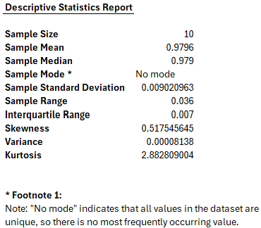
Figure 1 Example of Descriptive Statistics
It’s important to note that this approach is not limited to academic research. In forensic practice, descriptive statistics are also used in examination reports to objectively summarize evidence, communicate findings clearly, and support expert conclusions, a practice underscored by Aitken and Taroni in their discussion on the evaluation of forensic evidence [2]. Whether you’re writing a research article or a forensic examination report, descriptive statistics help ensure your results are transparent, understandable, and defensible.
Now that we’ve seen an example of descriptive statistics in action (Figure 1) let’s examine each statistic in more detail and consider how it contributes to our understanding of the data.
Descriptive Statistics Explained: A Forensic Perspective
Descriptive statistics are essential tools for summarizing and interpreting quantitative data, especially in research and forensic examinations. They provide a snapshot of our dataset’s main features, making complex information understandable and actionable. Below, we explain each statistic using our example data.
Understanding Each Descriptive Statistic
- Sample Size:
- Definition: The total number of observations or data points in our dataset.
- Example: 100
- Why it matters: The sample size indicates the amount of data analyzed and impacts the reliability of the findings.
- Sample Mean:
- Definition: The average value of all observations in the dataset.
- Example: 2212.36
- Why it matters: The mean gives us a central value around which the data points cluster.
- Sample Median:
- Definition: The middle value when all observations are ordered from smallest to largest.
- Example: 2070.5
- Why it matters: The median is less affected by extreme values (outliers), providing a robust measure of central tendency.
- Sample Mode:
- Definition: The value that appears most frequently in the dataset.
- Example: 1984.0
- Why it matters: The mode identifies the most common value, which can be useful for spotting patterns or anomalies.
- Sample Standard Deviation:
- Definition: Measures how spread out the values are from the mean.
- Example: 453.95
- Why it matters: A higher standard deviation indicates greater variability in the data.
- Sample Range:
- Definition: The difference between the highest and lowest values in the dataset.
- Example: 1882.0
- Why it matters: The range gives us a quick sense of the spread of our data.
- Interquartile Range (IQR):
- Definition: The range of the middle 50% of our data (from the 25th to the 75th percentile).
- Example: 207.25
- Why it matters: The IQR is less sensitive to outliers and provides a clearer picture of the central data spread.
- Skewness:
- Definition: Measures the asymmetry of the data distribution.
- Example: 1.98
- Why it matters: Positive skewness (as here) means the tail on the right side is longer; negative skewness means the left tail is longer. Skewness helps us understand if our data is biased toward high or low values.
- Variance:
- Definition: The average of the squared differences from the mean.
- Example: 206067.49
- Why it matters: Variance is another measure of data spread, but it is less intuitive than standard deviation because it is in squared units.
- Kurtosis:
- Definition: Measures the “tailedness” of our data distribution (how heavy or light the tails are compared to a normal distribution).
- Example: 2.89
- Why it matters: Kurtosis helps us detect the presence of outliers. A value near 3 is typical for normal distributions; higher or lower values indicate different tail behaviors.
Why These Statistics Matter in Forensic Research
Descriptive statistics help us summarize our data, identify patterns, detect anomalies, and communicate findings clearly in research papers, forensic reports, or presentations. Understanding and reporting these statistics ensures our conclusions are transparent, defensible, and evidence-supported.
Hands-On Example: Calculating Descriptive Statistics for Image Similarity
Let’s put theory into practice with a hands-on example using a simulated dataset of Pearson Correlation Coefficient (PCC) scores. These scores measure the similarity between 10 original images and their slightly altered copies. In forensic multimedia analysis, such comparisons are common when assessing whether images have been tampered with or differ due to compression or noise.
How to Use the Example Spreadsheet
- Download the Spreadsheet:
You can find the provided
.xlsxfile in the GitHub repository. Download it to your computer. - Enter Your Data:
- Column A: Paste your own PCC scores (or use the pre-loaded example).
- Pre-loaded Example:
- Example Dataset
0.985 0.982 0.980 0.978 0.977 0.976 0.975 0.999 (outlier) 0.963 (outlier) 0.981 - Optional Instructions
If you have your own data you want to use up to 100 entries in one column, you can use the following instructions.
Instructions:
- Paste your data in Column A (A2:A11).
- View the calculated statistics in the adjacent columns.
- Experiment by changing the values to see how the statistics update.
Conclusion
In this hands-on example, we calculated and reported the basic descriptive statistics for a set of simulated Pearson Correlation Coefficient (PCC) scores, illustrating how these measures help summarize and interpret image similarity data. By following standard reporting conventions, we would present these descriptive statistics, such as sample size, mean, median, mode, standard deviation, range, interquartile range, skewness, variance, and kurtosis, in the Results section of a research paper or forensic examination report. I prefer to present this data in a table for clarity and ease of reference.
In the Discussion section, we would then dig deeper into the meaning of these statistics, exploring what they reveal about the data’s central tendency, variability, and distribution. We will expand on these descriptive findings to further enhance our understanding by visualizing the data using box plots (to highlight range and IQR) and bell curves (to illustrate skewness, variance, and kurtosis). These visual tools help reveal patterns and outliers that simple numerical summaries may not fully capture.
Stay tuned for our next post, where we will explore these advanced descriptive statistics and data visualization techniques!
References
[1] Lucy, D. (2005). Introduction to statistics for forensic scientists. John Wiley & Sons.
[2] Aitken, C., & Taroni, F. (2004). Statistics and the evaluation of evidence for forensic scientists (2nd ed.). Wiley. https://doi.org/10.1002/0470011238